A few days ago, I wrote a crawler (with NodeJS and Sequelize) that fetches publicly available data from GitHub’s GraphQL API. More precisely, I downloaded information about users, repositories, programming languages and topics.
After running the crawler for a few days, I ended up with 154,248 user profiles, 993,919 repositories and 351 languages, many of which I had never heard of (e.g. did you know about PogoScript?). However, although my MySQL database is already 953 MB in size with only these data, I barely crawled 0.4 % of all user profiles (~ 31 million).
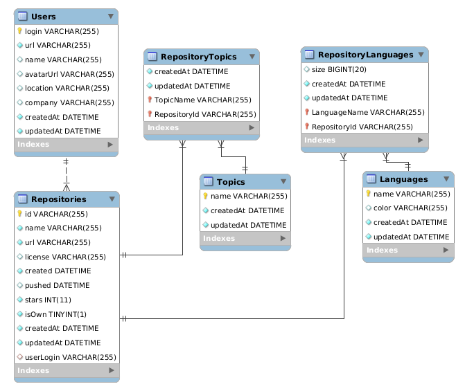
The first (less extensive) version of my database – which I performed the following analyses on – looked like this.
While one could argue that the data I collected is not of a representative sample size, I still wanted to do some data analysis on it – just for fun.
Analyses
To perform the analyses, I used Python 3 with Pandas and Matplotlib.
1
2
3
4
5
6
7
8
9
10
11
12
import apriori import pymysql import pandas as pd import matplotlib.pyplot as plt from sqlalchemy import create_engine
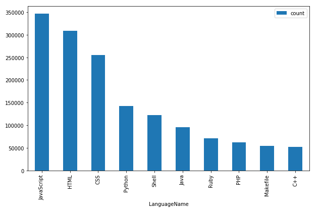
One of the first and most obvious thing to check (for the sake of brevity I’ll skip basic data set statistics like count, mean, variance, …) is which languages are most widely used.
1
2
3
4
5
6
7
df_top_langs = pd.read_sql_query('''
    select LanguageName, count(LanguageName) as count from RepositoryLanguages
    group by LanguageName
    order by count(LanguageName) desc
    limit 10;
''', con=connection)
df_top_langs.set_index('LanguageName').plot.bar(figsize=(12,8))
Not too surprisingly, the typical web stack consisting of JavaScript, HTML and CSS, is among the most popular programming languages, according to how often they appear in repositories.
Least popular programming languages
A little more interesting is to see, which programming languages occur least.
1
2
3
4
5
6
7
df_last_langs = pd.read_sql_query('''
    select LanguageName, count(LanguageName) as count from RepositoryLanguages
    group by LanguageName
    order by count(LanguageName) asc
    limit 10;
''', con=connection)
print(df_last_langs)
Here are the results. Have you heard of any one of them? I didn’t.
Let’s analyze the users’ skills in terms of languages. I decided to consider a user being “skilled” in a certain language if at least 10 % of her repositories’ code is in that language.
What I wanted to look at is combinations of different skills, i.e. languages that usually occur together as developer skills. One approach to get insights like these is to mine the data for association rules, e.g. using an algorithm like Apriori (as I did). The implementation I used was asaini/Apriori.
The left part of each row is a tuple of tuples of programming languages that represent an association rule. The right part is the confidence of that rule.
For example: Read ((('ShaderLab',), ('C#',)), 0.904) as “90 % of all people who know ShaderLab also know C#”.
The results reflect common sense. For instance, the rule that developers, who know VueJS, also know JavaScript seems to make sense, given that VueJS is a JavaScript framework. Analogously, CMake is a common build tool for C++, etc. Nothing too fancy here, except for that I didn’t know about ShaderLab and GLSL.
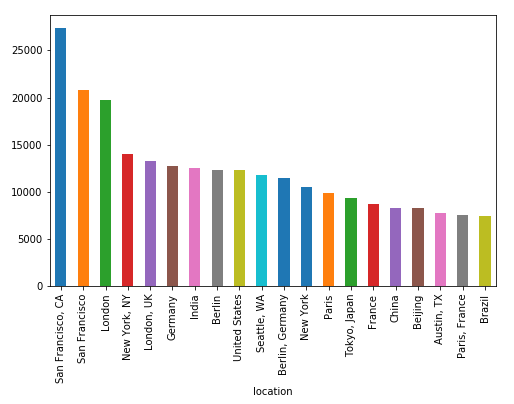
Locations
Let’s take a look at where most GitHub users are from. Obviously, this only respects profiles where users have set their locations.
deflanguage_replace(df): df = df.copy() # Little bit of manual cleaning replace = {'San Francisco': 'San Francisco, CA', 'Berlin': 'Berlin, Germany', 'New York': 'New York, NY', 'London': 'London, UK', 'Beijing': 'Beijing, China', 'Paris': 'Paris, France'} for (k, v) in replace.items(): ifisinstance(df, pd.DataFrame): if k in df.columns and v in df.columns: df[k] = df[k] + df[v] df = df.drop([v], axis=1, errors='ignore') else: if k in df.index and v in df.index: df[k] = df[k] + df[v] #df = df.drop([v], axis=1) del df[v] return df
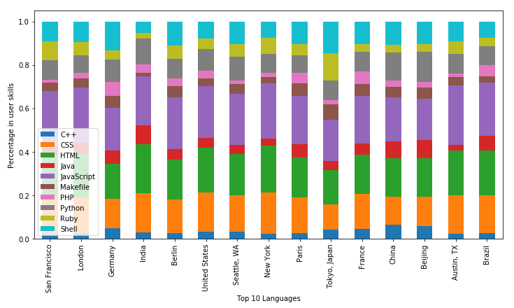
langs_by_loc = {} for l in df_locations.index: langs_by_loc[l] = df1[df1['location'] == l][['LanguageName']].groupby('LanguageName').size() df_loc_langs = pd.DataFrame.from_dict(langs_by_loc).fillna(0)
df_loc_langs = language_replace(df_loc_langs) df_loc_langs = df_loc_langs.T df_loc_langs = df_loc_langs.drop([c for c in df_loc_langs.columns if c notin df_top_langs['LanguageName'].values], axis=1)
Look like there are no real outliers in the distribution of developer skills between different cities of the world. Maybe you could say that, e.g., Indians like web frontends a little more than command-line hacking.
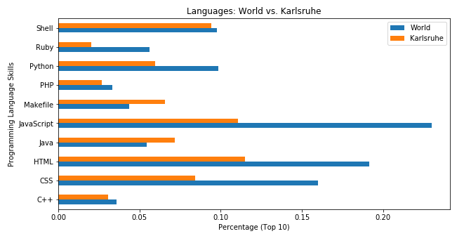
Skills: Karlsruhe vs. the World
While an overview is cool, I found it even more interesting to specifically compare between to cities. So in the following chart I compare language-specific programming skills in Karlsruhe (the city where I live and study) to the rest of the world’s average.
These results are a bit surprising to me. Clearly, Karlsruhe-based developers seem to dislike JavaScript compared to the world. However, this is different from what I experienced in several student jobs and internships here.
Project Tech Stacks
Last but not least, let’s apply Apriori once more, but this time in a slightly different way. Instead of looking at user skills, let’s look at languages that occur together on a per-repository basis. And instead of trying to find rules, let’s only look at frequent item sets (which are the basis for rules). My expectation was to get back sets of commonly used tech stacks.
Here, the left side is sets of frequently occurring combinations of languages. The right side is the set’s support, which is the relative occurrences of that set among the whole data set. Obviously, many of these are actually common “tech stacks” and almost all of them are web technologies. I guess GitHub is most popular among web developers.
Conclusion
There is a lot of more complex analyses that could be might on rich data like this and probably tools like BigQuery are better suitable than Pandas, operating on a tiny sample. However, I used this little project to improve my EDA skills and hopefully give you guys an interesting article to read. Let me know if you like it!